


TDS Project
Introduction to the TDS analysis tool package (Version 2017.08)
Transcriptional Disease Signature (TDS) analysis tool package is a set of custom R projects that implement a “shiny” server to deliver a user-interface (UI). The UI can be launched remotely through shiny.io, or locally by downloading the tool package stored on GitHub through the “shiny” R package. There are three tools in the package: “TDSNormalization” normalizes raw gene expression counts generated from the NanoString nCounter platform; “DEGAnalysis” calculates mean and variance as well as performs differential expression analysis; and “TDSScore” evaluates the effect of treatments on TDS gene expression.
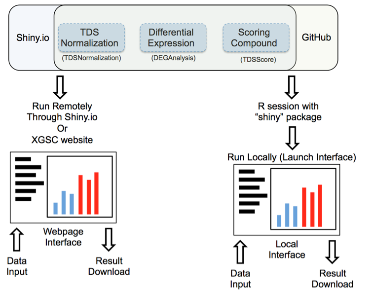
Figure 1: Launching interface through shiny.io or GitHub
Launch interface through shiny.io
Shiny.io is an R server dedicated to hosting shiny projects. Launching the TDS analysis tool interface through shiny.io does not require any command line input; the interfaces are accessible by clicking: “TDSNomalization”,”DEGAnalysis”, or ”TDSScore” on http://www.xiphophorus.txstate.edu/resources/tdsproject webpage, or directly launched through the following URLs:
“TDSNormalization”: https://tdsprojectylu.shinyapps.io/TDSNormalization/
“DEGAnalysis”: https://tdsprojectylu.shinyapps.io/DEGAanalysis/
“TDSScore”: https://tdsprojectylu.shinyapps.io/TDSScore/
The chosen UI will be launched in your web browser.
Launch interface through GitHub
TDS analysis tools are stored on the GitHub website “https://github.com/3402bioinformaticsgroup/”. For users who have access to R, the TDS analysis tool interface can also be launched through R. Launching the UI through GitHub requires minimum script experience in the R environment. Some of the functions are only available through local servers at this stage of development, for example, download of the pdf normalization report. Additionally, since the server source code is downloaded to your local workstation, users can customize the server and fine-tune the data analysis pipeline.
To start the UI in R:
# install.packages(‘shiny’)
# library(‘shiny’)
# shiny::runGitHub('TDSNormalization','3402bioinformaticsgroup')
# shiny::runGitHub('DEGAanalysis','3402bioinformaticsgroup')
# shiny::runGitHub('TDSScore','3402bioinformaticsgroup')
Each UI requires two R files, ui.R and server.R. Once the above command is executed, the ui.R and server.R files of selected tool will be downloaded to your local workstation. The user workstation will then be used as a server to host the TDS analysis tools. The UI will be launched in a web browser locally.
To terminate a tool, press ESC on the R command interface.
GitHub allows user to report bugs/problems, feel free to do so if you find any glitch, or contact Xiphophorus Genetic Stock Center for assistance.
Input file format
All input files for the TDS tool package must be in comma-delimited format (.csv). The tool package only outputs .csv format files and .pdf reports. Sample input files are stored in GitHub directory dedicated for each tool. User input files need to follow the format of sample files. In short, the input data needs to be in a matrix, with columns as samples, and rows as probes; column names are unique sample names, and row names are unique probe names. The content of the matrix can be raw counts, normalized counts or LogFC values. For details, see instructions for each tool.
The output file from NanoString is in .RCC format – a specialized comma delimited format. The .RCC files can be converted to a .csv file manually, or by using NanoString’s R package “NanoStringNorm”. The XGSC also has its own .RCC data wrapper. Please contact us if you are interested.
TDS analysis tool package instructions
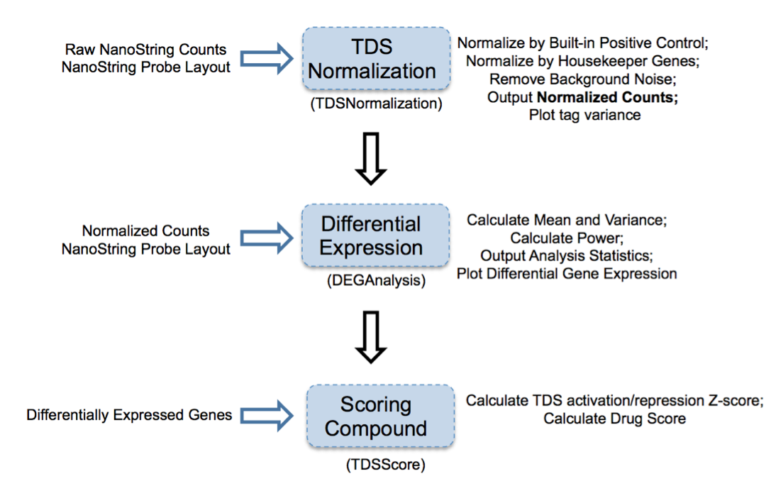
Figure 2: Overview of TDS analysis tool package
TDS are a set of genes that hallmark transcriptional change of a biological condition (e.g., disease) relative to another condition (e.g., normal). The purpose of accessing TDS expression changes after treatment with select compounds is to use gene expression as a marker to screen compound(s) and identify the one(s) that can shift TDS pattern to normal state.
1. TDSNormalization
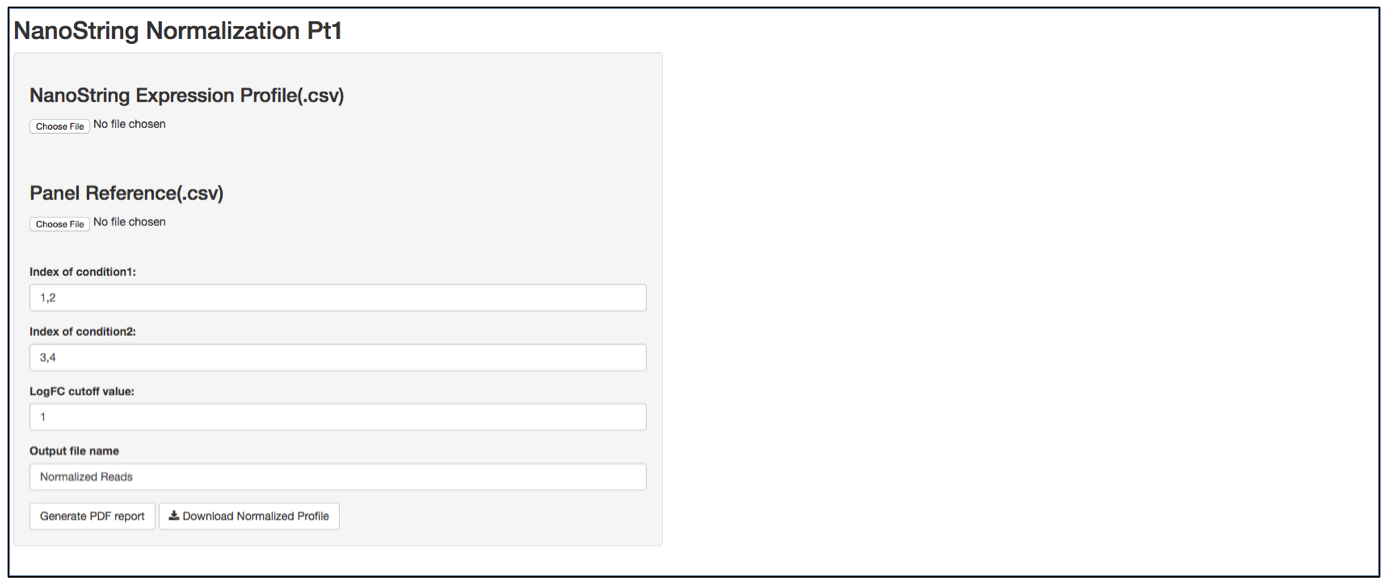
a. Launch user interface through shiny.po or GitHub
b. Click “Choose File” under “NanoString Expression Profile(.csv)” and select the raw count (.csv) file you want to upload. The raw count (.csv) file needs to have column names as sample names, and row names as probe names with numeric values in the data matrix. The first 5 rows of input data will be shown to the right of the UI.
c. Click “Choose File” under “Panel Reference (.csv)” and browse to the panel reference (.csv) file. This file should include header information and the type of probes in very first column. Usually, NanoString names custom probes as “Endogenous”, built-in positive and negative control probes as “Positive” and ”Negative”, and custom housekeeper probes as “Housekeeping”. The order of the probes should be the same as the order in the raw count (.csv) file.
d. It is not necessary to define the column index of “conditon1”, “condition2” and LogFC cutoff value, as the normalization will be performed on all input data.
e. Define the output file name for the normalized gene expression, it is not necessary to include “.csv” at the end of the file as the file format is automatically attached to the output file name.
f. The program should automatically start normalization process once it collects all required information. Once finished, 3 plots will be generated on the right of the UI: CV% of raw data, CV% of processed data, and density of CV% throught the data normalization pipeline. CV% is calculated from all samples, therefore comparing CV% of one probe to another is meaningless as genes that are differentially expressed between two biological conditions tend to generate a larger CV%. In contrast, comparing the CV% of the same probe before normalization and after normalization provides how much variation from the assay has been removed. TDSNormalization does not disgard any control probes from the normalization process, therefore the user needs to determine what is an appropreate cut-off value. After normalization, the CV% of housekeeper genes are expected to be small. It is recommented that the whole dataset be re-normalized after any housekeeper gene that has a CV% larger than 30% is removed from raw data file and corresponding panel reference file. The output file also includes a .pdf normalization report that includes all the normalization statistics after each normalization step. Besides housekeeper genes CV% mentioned above, postive control scaling factor is another parameter. A scaling factor is a measurement of hybridization efficiency for a specific sample slot. A value between 0.3 and 3 are recommended by NanoString as normal. If you observe a scaling factor much larger than 3 or much smaller than 0.3, consider re-running the sample.
2. DEGAnalysis
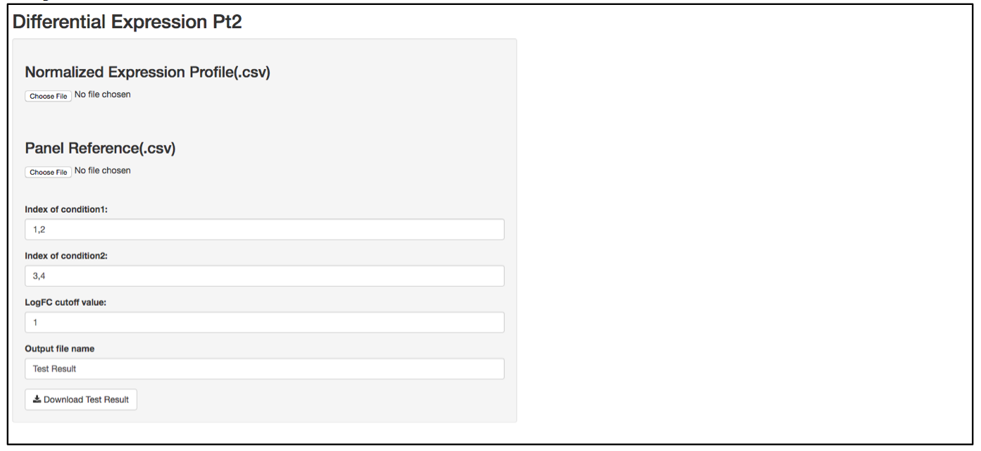
a. Launch user interface through shiny.po or GitHub
b. Click “Choose File” under “Normalized Expression Profile (.csv)” and browse to the normalized expression profile (.csv) file you want to upload. The normalized expression profile (.csv) file needs to have column names as sample names, and row names as probe names, with numeric values in the data matrix. The column names (i.e., sample names) of input data will be showed on the right of the UI.
c. Click “Choose File” under “Panel Reference (.csv)” and browse to the panel reference (.csv) file. This file should include the type of probes as the very first column, and header information. This panel reference file is the same as what was used in the normalization step. The order of the probes should be exactly the same as the order in the raw count (.csv) file. If any housekeeper genes were removed, make sure the correct panel reference file is uploaded.
d. In the text box under “Index of condition1” and “Index of condition2”, define the column index for conditon 1 and condition 2 according to the input data preview. Differential expression is tested on condition 2 over condition 1, so it is recommended to set condition 1 as control and condition 2 as treated. Column indices should be delimited by comma. For example, if control samples are in column 1, 2, 3, and 4, type 1,2,3,4 in “Index of condition1”.
e. When defining the output file name for the statistics analysis result, it is not necessary to include “.csv” at the end of the file as the file format will automatically be attached to the output file name.
f. The program should automatically start calculating test statistics. Statistical parameters (i.e., mean, standard diviation, sample size, effective size, test power, logFC, p-value, required sample size at current effective size with a power of 0.8) are included in the output test result file.
g. After the analysis is complete, two plots will be generated on the right side of the UI; one plot shows the required sample sizes to identifiy certain logFC given the variation in the dataset, at a significant level (0.05) with different power. Users can use this plot to estimate what is an appropriate logFC and re-adjust the logFC cutoff for the analysis.
3. TDSScore
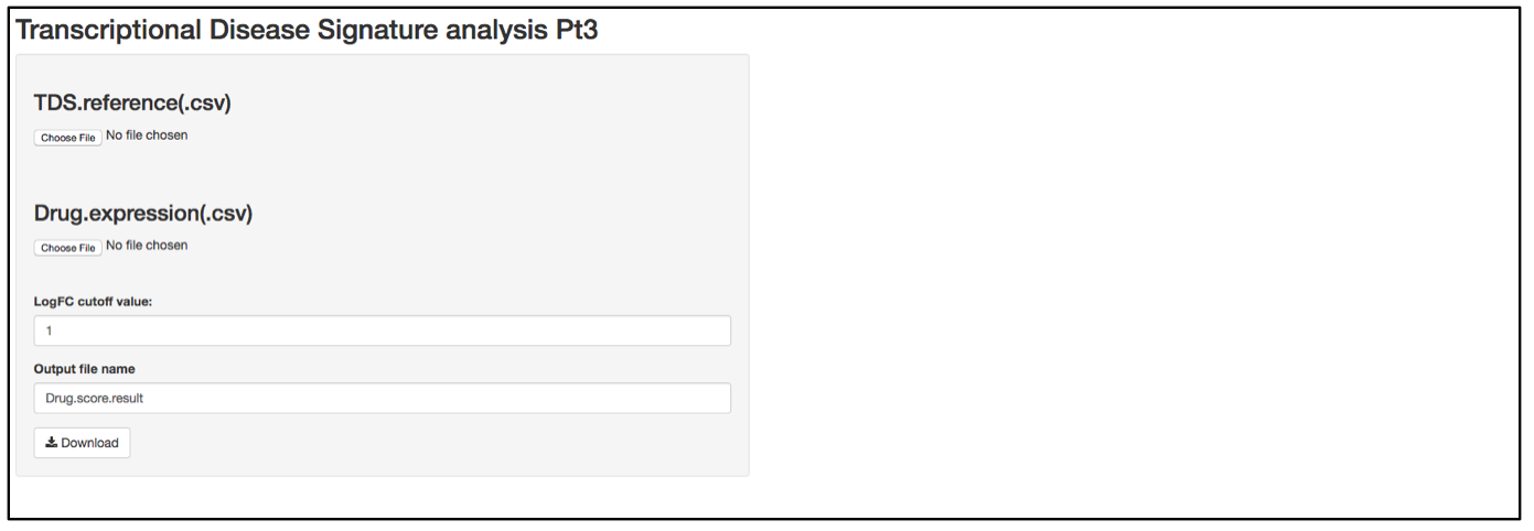
a. Launch user interface through shiny.po or GitHub
b. Click “Choose File” under “TDS.reference (.csv)” and browse to the TDS.reference (.csv) file. This file needs to have column names as feature names, and row names as probe names. This file serves as an annotation of the TDS probes and includes all the information related to the corresponding genes. Column 1 is the AUC of ROC curve in the genome profiling experiment in which TDS genes were selected. This value represents a false positive rate in the initial test and serves as weight for differential expression. Column 2 and Column 3 are names and description of the TDS genes. Column 4 includes the Log2FC of the TDS genes in the initial test.
c. Click “Choose File” under “Drug expression (.csv)” and browse to the differential expressed gene list (.csv). This file should have column names as sample names (i.e., compound names), and row names as probe names, with numeric values in the data matrix. The first 5 rows of this input data will be shown on the right of the UI. If users have a matrix of logFC that were generated by different compound treatments, the user needs to replace any logFC that has a p-value larger than cut-off (e.g., 0.05) replaced by 0.
d. In the text box under “LogFC cutoff value”, define the logFC cut-off value. Any logFC value that is between logFC and –logFC within the input matrix will be replaced by 0.
e. When defining the output file name for the drug score result, it is not necessary to include “.csv” at the end of the file as the file format is automatically attached to the output file name.
f. The program should automatically start calculating the TDS activation Z-score and drug score. These parameters are included in the output test result file.
g. After the analysis is complete, there will be two plots generated on the right side of the UI. One plot shows the TDS activation Z-score. Activation Z-score is used to determine whether a compound works as an activator (i.e., further change TDS expression to a direction that is different from normal) or repressor (i.e., shift TDS expression to a state that is similar to normal) of TDS expression. It is calculated based on an algorithm applied in Ingenuity Upstream Analysis (IPA, Qiagen, Redwood City, California). Briefly, we took a statistical approach by defining a Z-score that determines whether a compound is a significantly more “activated” TDS than “repressed” TDS (z>0) or vice versa (z<0). Here, significance means that we reject the hypothesis that the overall compound effect on TDS expression is random with equal probability. The distribution underlying this null hypothesis is defined by a random variable:
![]()
where +1 corresponds to an activated state and -1 to an inhibited state, and both values are chosen with probability 1/2. The index i runs from 1 to N with N being the number of TDS. Let:
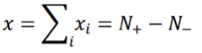
where N+/- are the number of “activated”/”inhibited” TDS and N+ + N- = N. The variance of xi is σ2 = 1, so the variance of x is given by:
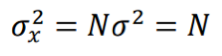
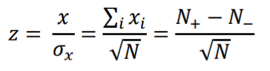
and the z-score statistic (with mean equal to zero and variance equal to 1) is defined by:
Another score (i.e., drug score) is calculated using a random-walk model and is plotted on another graph on the right side of the UI. Kolmogorov-Smirnov statistic utilized in Connectivity Map (https://portals.broadinstitute.org/cmap/) and Gene Set Enrichment Analysis (http://software.broadinstitute.org/gsea/index.jsp) is adapted to rank the effectiveness of compounds in “activating” or ”repressing” TDS expression. For each compound treatment i in a collection of c total compounds, the Kolmogorov-Smirnov statistic is computed for both up-regulated genes and down-regulated genes in the TDS, giving ksiup and ksidown. Let n be the number of the TDS and t be the number of compound related differentially expressed genes. Order all n TDS by the extent of their expression change for the current instance i. Construct a vector V of the position (1... n) of each differentially expressed genes in the ordered list of all TDS and sort these components in ascending order such that V(j) is the position of differentially expressed gene j, where j = 1, 2, ..., t. Then compute the following two values:
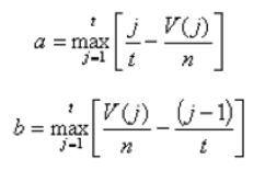
If a > b, set ksi = a. Set ksi = -b if b > a. The up scores and down scores are ksiup and ksidown, respectively. These values are reported on the result table as "up" and "down". The score Si is set to zero where ksiup and ksidown have the same sign. Otherwise, set si to be ksiup - ksidown, p to be max( si) and q to be min( si) across all instances in the collection c. The score Si for the remaining instances is defined as si/p, where si > 0, or -(si/q), where si < 0. The "score" values are reported on the detailed result table.
The TDS analysis tool package and hosting server are being constantly maintained. Update information is available through GitHub version control. Please feel free to contact us if you have questions, run into problems when using TDS analysis tool package, or need bioinformatics/machine learning solutions for your project.